

Democrats did well in the 2026 midterm elections. According to the current tally, they gained 41 House seats, eight Senate seats, and five governorships. Democratic candidates of all types had success, making it difficult to easily point the finger at this or that faction for blowing the election.
This has generated some frustration among factional partisans because such partisans are heavily invested in the idea that their style of politics is electorally superior to the politics of other factions. They can't point to winners and losers to support their positions because, in this election, everyone was a winner. So they are forced to make their case by analyzing margins of victory, which is hard to do well and full of uncertainty even when it is done well.
In this piece, I walk through various approaches to quantifying candidate-specific performance to provide a sort of primer on how to think about this and successfully navigate the deluge of election pseudo-statistics.
I. Raw Vote Share
The most obvious, though naive, way to distinguish between winners is to look at their raw vote share. If one Democratic candidate won 51 percent of the votes cast in their race and another won 70 percent of the votes cast in their race, then, at a glance, it seems like you could say that the 70-percent candidate performed better than the 51-percent candidate.
Certainly the 70-percent candidate did better, but this is not the same thing as performing better. When pundits talk about performance, they are trying to isolate the effect the candidate's own characteristics had on the election results. Raw vote shares do not do this because raw vote shares reflect other factors as well, including the underlying tendencies of the voters in that area. In other words, it's possible that the 70-percent district leans more Democratic, and the 51-percent candidate would have also gotten 70 percent in that district.
II. Expected Vote Share
To isolate the candidate-specific effects, you have to establish some kind of baseline figure for what the election results would have been in a hypothetical version of the race where the candidate was a "generic" Democrat. The difference between the actual results and these "expected" results is then assumed to reflect the unique characteristics of the candidate.
This is not an easy thing to do, and most of the efforts I see in the discourse are ridiculous.
A. Uniform Swing as Expected Vote Share
The most common approach to quantifying expected vote share is to determine how vote shares changed nationally from the prior election and then assign that change uniformly across every voting area in the country. This is what Kevin Deluca did in the following graph.
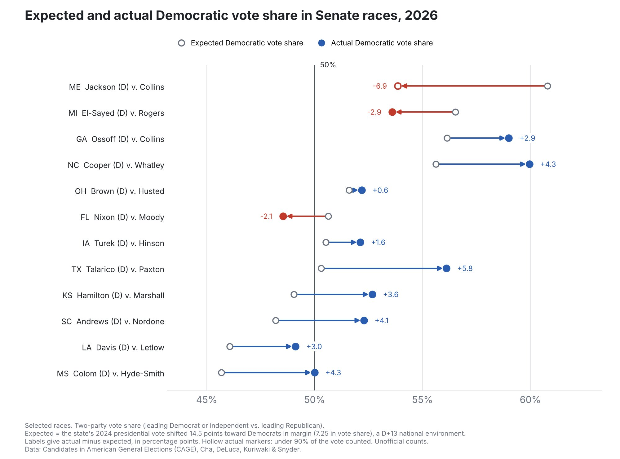
It may look sophisticated, but, as the caption explains, all Deluca did was go through each of the twelve states and add 7.5 points to Harris's 2024 presidential result in that state. This is his entire model for expected vote share. The difference between this expected vote and the actual vote is then used to declare underperformers and overperformers.
The simplicity of this model is very charming and no doubt explains why I see it more than any other: anyone who can add and subtract is capable of running the model. But does it really make sense to suppose that, if you ran a generic Democrat in every Senate race in the country, each of them would have received a Harris+7.5 vote share?
Even if one were to suppose that all of the non-candidate differences between these states and races could be fully captured by Harris's 2024 presidential result, why would equal performances by generic Senate candidates show up as equal changes in percentage points? Wouldn't it make more sense for equal performances to show up as equal changes in percent of the 2024 non-Democratic share that was converted to the 2026 Democratic share?
To see what I mean, imagine two House districts, one where Harris got 80 percent of the vote in 2024 and another where Harris got 20 percent of the vote in 2024. If you put equally-performing generic Democrats in those districts, what would you expect the result to be?
The uniform-swing approach says that we should expect them to add the same number of percentage points. So, for example, we should expect the 80-percent district to become a 90-percent district and the 20-percent district to become a 30-percent district. In this scenario, both districts moved equally by 10 points. But to move 10 points in the 80-percent district, you have to persuade 50 percent of the non-Democratic voters. Moving 10 points in the 20-percent district only requires persuading 12.5 percent of the non-Democratic voters. Why would we expect one generic Democrat to be four times as persuasive as another generic Democrat? How is that equal performance?
The premise of the uniform-swing model, which is that equal performance equates to equal percentage points, is nonsensical on its face. Clearly, the number of points an equal performer can move will vary state to state and district to district by the share of the electorate that is even capable of being moved. Simple linear regressions using the House and Senate results provide some empirical support for this point.
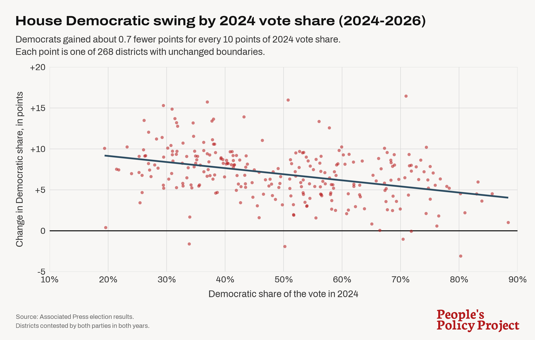
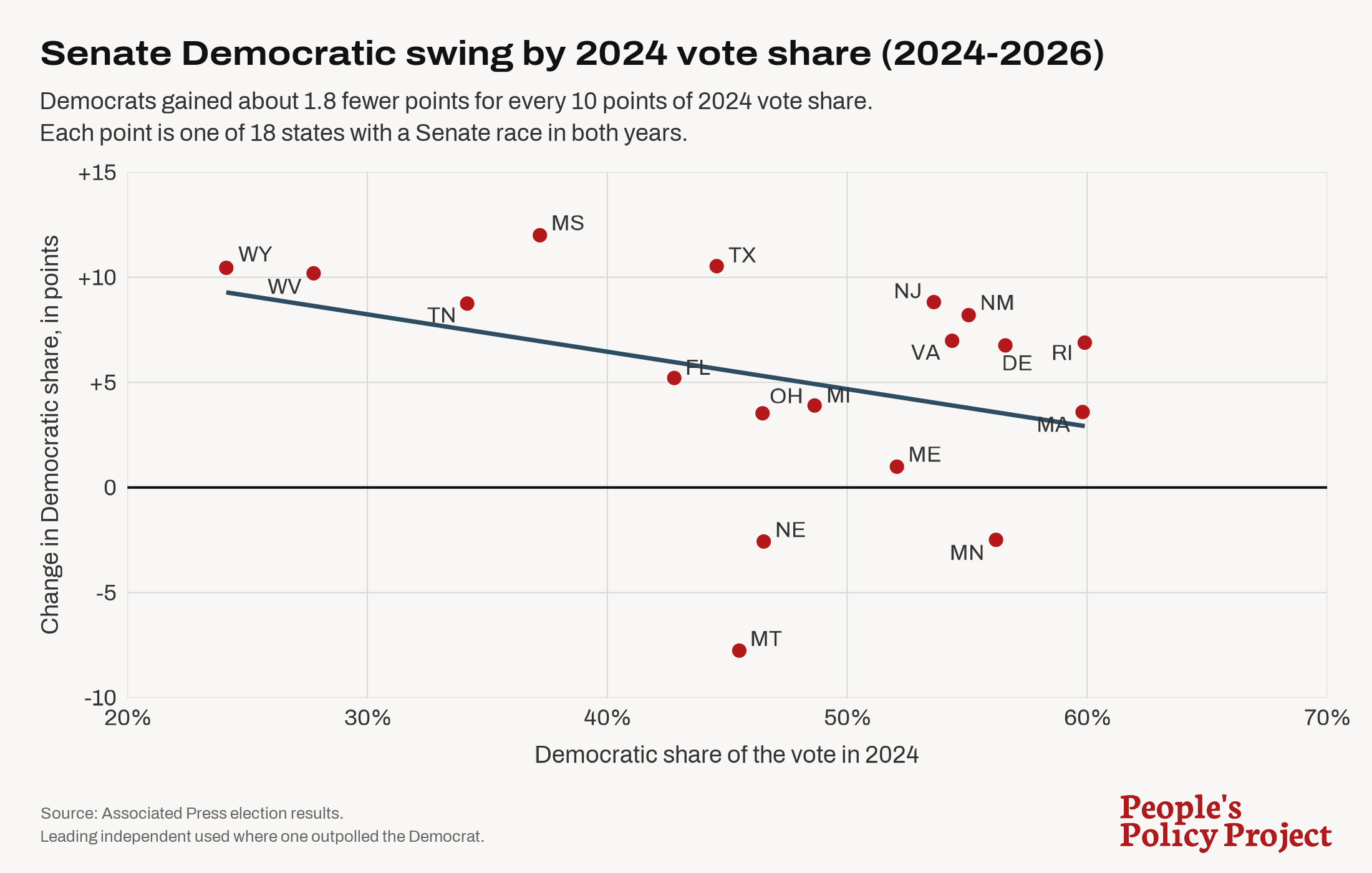
There are at least two other big problems with this approach to modeling expected vote share.
First, a uniform vote swing would make sense only if you were modeling generic Democrat versus generic Republican. But these Senate races do not have generic Republicans in them. Maine's Troy Jackson ran against a 30-year incumbent in Susan Collins while Texas's James Talarico ran against a scandal-plagued non-incumbent in Ken Paxton. The difference between actual vote share and expected vote share would capture the combined candidate effects of both the Democratic candidate and the Republican candidate.
So, for instance, if Troy Jackson runs 2 points behind the uniform-swing expected vote share, that could be because he has negative candidate effects, because Collins has positive candidate effects, or because of some combination of the two. Likewise, if Talarico runs 2 points ahead of the generic-versus-generic expected vote share, that could be because he has positive candidate effects or because Paxton has negative candidate effects. By construction, the uniform-swing approach assumes that the relative overperformance or underperformance of Republican candidates is uniformly zero.
Second, different districts have different demographic compositions, which should generate different swings even with equally-performing generic Democrats. For example, here's what percent of each racial group voted for the Dems nationally in 2024 and 2026.
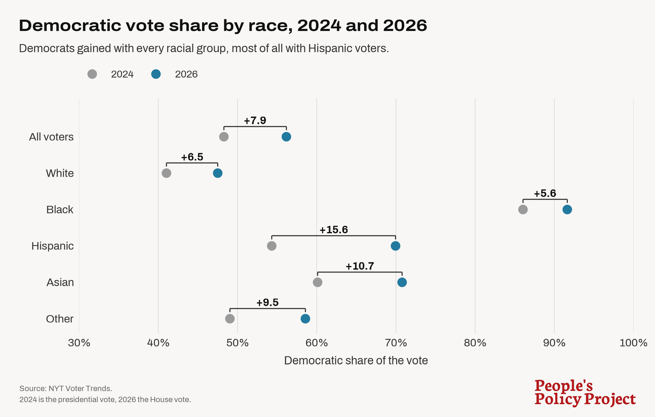
As we can see, the vote swing varies by racial group. Given this variation, the only way equally-performing generic Democrats would generate uniform vote swings in every voting district is if every voting district had the same racial demographics. They don't.
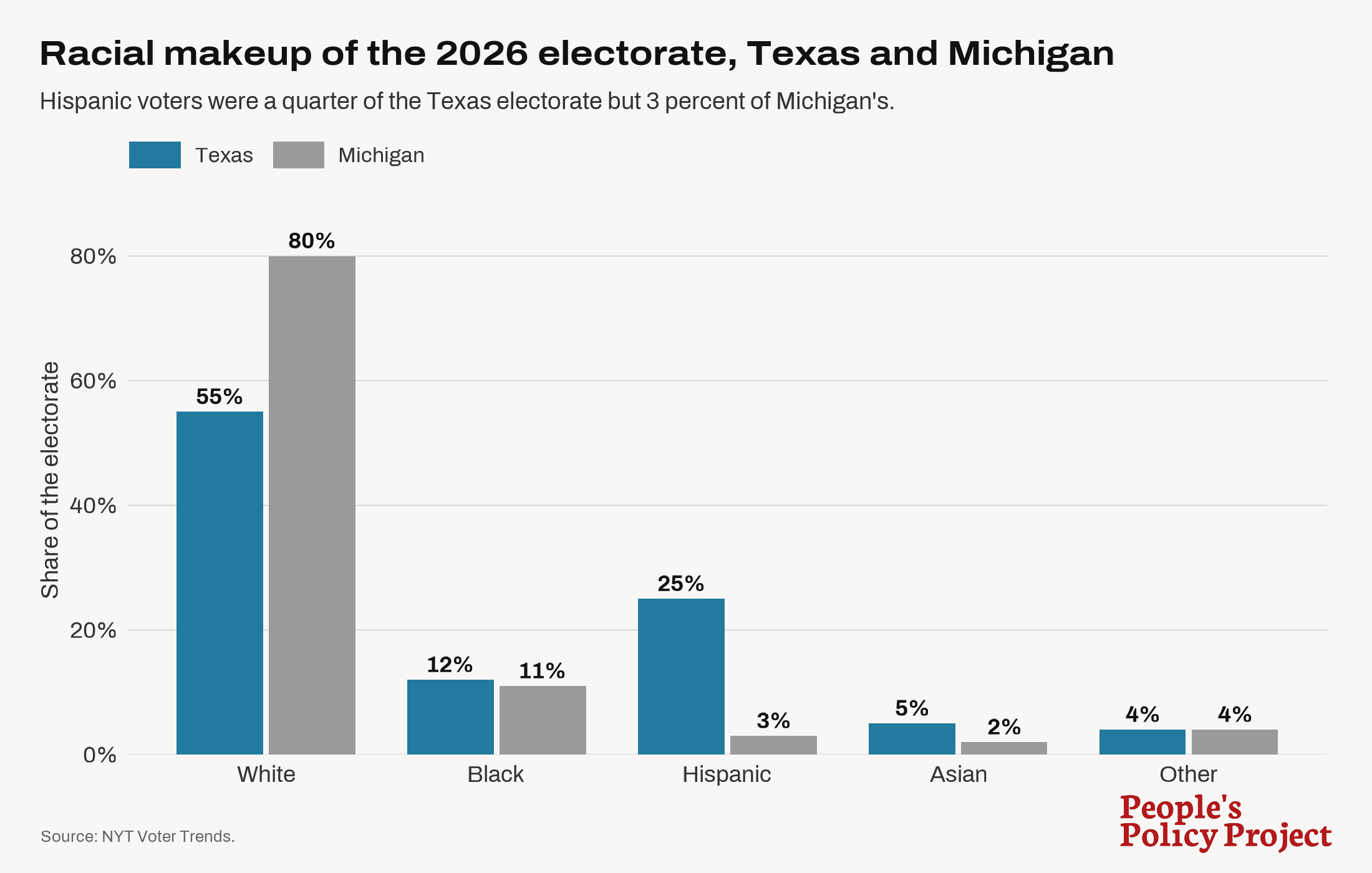
Race is the most obvious example, but other demographic variables like income and education vary across districts and also drive differential vote swings separate from anything having to do with candidate effects.
B. Overlapping Elections as Expected Vote Share
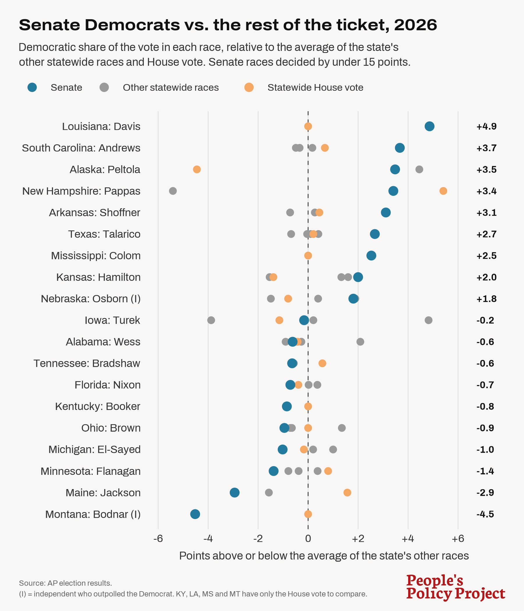
The second most common approach to quantifying expected vote share is to compare a specific Democratic candidate's vote share to the vote share of other Democratic candidates running for other positions within the same voting area. So, for instance, you might compare how one statewide candidate did to how other statewide candidates in that same state did.
This approach avoids some of the problems of the uniform-swing approach. It does not require us to clumsily extrapolate from prior election results. By construction, it controls for demographics and other sorts of variation between different groups of voters because it compares how different candidates did among the exact same voters in the same year. No longer are we stuck having to wonder whether Michigan-2024 is comparable to Michigan-2026 or whether Michigan-2026 is comparable to Texas-2026. Instead, this approach just compares Michigan-2026 to Michigan-2026.
But this overlapping-elections approach still has some of the same problems as the uniform-swing approach and some unique problems of its own.
Like the uniform-swing approach, the overlapping-elections approach effectively assumes that Republican candidates never underperform or overperform. But this is obviously untrue. In Texas, Senator-Elect Talarico (Dem) received 55.1 percent of the vote while Governor-Elect Hinojosa (Dem) received 52.8 percent of the vote. The overlapping-elections approach would say that Talarico overperformed by 2.3 points, or, alternatively, that Hinojosa underperformed by 2.3 points.
But these numbers don't allow us to reach any such conclusion. After all, another explanation would be that Talarico and Hinojosa performed exactly the same while Talarico's opponent, the scandal-plagued first-time Senate candidate Ken Paxton, underperformed by 1.15 points and Hinojosa's opponent, the 12-year incumbent Greg Abbott, overperformed by 1.15 points.
The overlapping-elections approach is also unable to determine the absolute quality of the candidates in a given geography, only their relative positions to one another (if that). The uniform-swing approach presumably uses national averages on the theory that a large sample across many geographies provides a more reliable indicator of what the average candidate quality is. But if your dataset only includes a handful of overlapping races, it's quite possible that a disproportionate share of the candidates in your dataset (even, potentially, all of the candidates in your dataset) are underperformers or overperformers. A Senator who runs slightly above a Governor or the combined House vote could be an overperformer, but they might also be an underperformer surrounded by even greater underperformers. This approach cannot distinguish between the two.
Another unique problem with the overlapping-elections approach is that it assumes that the only reason a voter would split their ticket — e.g. vote for a Democrat for Senator and then a Republican for Governor or House of Representatives — is because of the different characteristics of the candidates running in the various races.
But this is not true. A voter might also split their ticket because of differences in the powers of the various offices they are voting on. A voter who typically supports Republicans but dislikes Trump and wants to rein in his power may support a Republican for Governor while supporting a Democrat for the House. That same lean-Republican voter, while supporting a Democrat for the House, might support a Republican for the Senate, given that Senators serve six-year terms while all House representatives come up for re-election again in 2028.
Even if only a small percentage of voters think in this (quite rational) ticket-splitting way, it's enough to completely swamp most of the point differences we see in these overlapping-election results, especially when you add in the other problems identified above.
C. Regression Models
One of the least common approaches to quantifying expected vote share is also the most sophisticated: regression models. Rather than assuming a uniform swing or looking at overlapping elections, throw a variety of variables into a model that spits out an expected vote share for each geography. The difference between what the model outputs and the actual vote share is then presumed to be driven by candidate effects.
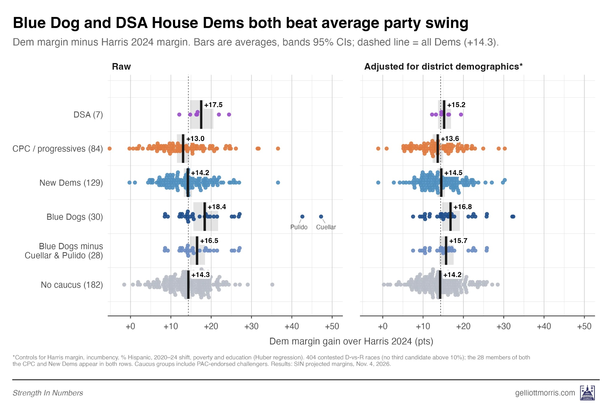
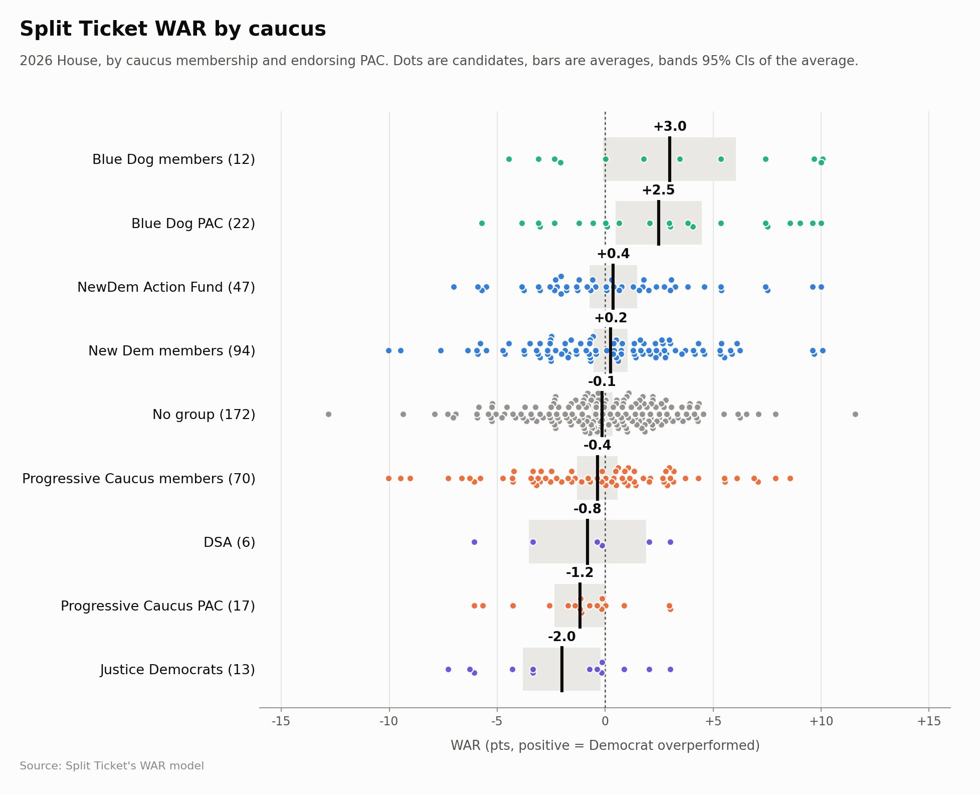
As far as I know, the two main sources for this approach are Split Ticket, which is now at The Argument, and Strength in Numbers led by G. Elliot Morris.
In this election, the Strength in Numbers approach showed no real difference between the various ideological groupings of House candidates. If anything, the DSA candidates overperformed the average Democrat.
Split Ticket, which uses a different regression model, reached a similar result, with only the Blue Dog PAC candidates (but not Blue Dog members) and Justice Democrat candidates posting performance results (slightly) distinguishable from zero.
The Economist also published the results of a model it apparently put together for the election. According to this model and its candidate groupings, moderates outperformed expectation by less than 1 point while progressives underperformed expectation by the same amount.
The main problem with this modeling approach is just that it is not totally clear what variables should be included in the models. This is why they all differ from one another.
Another problem, which plagues all of these expected-vote approaches, is that not all candidate effects are related to ideology. Candidates might do better or worse because of their identity, e.g. being a Muslim. They might do better or worse because of their personality, e.g. being charismatic or not. Indeed, as we can see in the scatterplots above, the differences between candidates in each bucket far exceed the average differences between the candidate buckets. This problem is especially relevant when it comes to candidate selection, e.g. when voting in a Democratic primary, because it suggests that the non-ideological aspects of candidates completely swamp the ideological aspects.
Arguably, these problems could be waved away if the various models all reached similar conclusions about candidate quality and did so at margins too large to plausibly deny. When it comes to the progressive-versus-moderates question, these three regression models do basically reach similar conclusions, which is a null conclusion. What departures we see from null in some of the models on some of the candidate groupings are so small that any grains of salt completely eradicate them.
III. Where That Leaves Us
Obviously, most discourse participants don't care about any of this and are happy to move around whatever chart they see that shows that science proves their politics is the best politics. But among pro-moderate pundits who do care at least some about maintaining a defensible argument on the merits, what I have seen lately is a proposal of sorts in which pro-progressive pundits agree that moderates do better than progressives in exchange for pro-moderate pundits agreeing that the gap is very small. Both Jonathan Chait and Matt Yglesias have gone this route after the election. In more recent exchanges I've had with Yglesias, he seems to retreat a bit further toward acknowledging that the moderate advantage can't be reliably demonstrated in the data but that it rests on strong theoretical foundations.
The problem with these strategic retreats is that the difference between zero and nearly-zero is not going to be big enough to convince anyone to abandon policy initiatives that they think are important, especially given that policy popularity changes over time in part due to the advocacy of policy partisans. If the current electoral penalty of advocating single-payer health care over expanding Obamacare subsidies is one point or less, it would be crazy for someone who believes single-payer health care would dramatically improve society to give it up, especially when the alternative of attempting to persuade some voters to change their minds on that, which includes running candidates who argue for it, also exists.